Model Building
Overview
We summarize the statistics of world cups from 1990 to 2018 for all the countries that made to the World Cup to help us make preditions of wining in the 2022 World Cup.
We tried different ways for model selection, including stepwise selection, forward and backward selection, and LASSO, with different selecting criterias, such as AIC, BIC, and p-values. After comparing the rmse, R-square and p-values, we decide to use the model from forward selection with p-value.
While there are two variables that are on the borderline of our threshold, alpha = 0.05, we got three different models to include either or both of these two variables. Then, we used cross validation to check which model has the best performance.After comparing their rmse, we get the final model - w = -1.554369 + 0.661219pld - 0.622216d + 0.015920rank + 0.153794gf -0.225378ga.
Potential predictors
VARIABLES AND DEFINITIONS
country: Individual country (represents national soccer
team)
part: Number of times each country has participated in
the World Cup (all time)
pld: Number of games played in the World Cup (since
1990)
w: Number of soccer games a country has won in the World
Cup (since 1990)
d: Number of soccer games a country has drawn in the
World Cup (since 1990)
l: Number of soccer games a country has lost in the
World Cup (since 1990)
gf: Number of goals a country has scored against
opponents in the World Cup (since 1990)
ga: Number of goals scored against a country in the
World Cup (since 1990)
gd: Goal difference of country (goals scored by country
minus goals scored against country)
pts: Number of points accumulated by country in the
World Cup (since 1990)
rank: Country Official FIFA ranking (2022 Rankings)
player: Name of top record goal scorer
goals: Number of goals scored by top record goal
scorer
land_area_km: Total area of the land-based portions of a
country’s geography (measured in square kilometers, km²)
confederation: Country FIFA confederation
Correlation Plot
In the dataset, we had 14 variables and 79 observations. To check for
collinearity, we use correlation plots to explore the relationship
between each pair of numeric predictors. To only include the numeric
variables, we use the select function to exclude the
qualitative variables, such as player, country, and gd. The deeper color
in the plot means stronger correlation between the two variables.
data <- read.csv("./data/worldcup_final.csv") %>%
  na.omit() %>%
  select(-country)
num = data[2:14] %>%
  select(-gd, -player)
corrplot(cor(num),  diag = FALSE)
Cross-validation
We decided to use forward selection for our final model, where we start with only the intercept and add one predictor at a time. The criteria we chose is p-value, which means we will select predictors to include based on p-values, until no more predictors having p-value less than 0.05 can be added to the model. While there are two variables that are on the borderline of our threshold, alpha = 0.05, we created three different models to include either or both of these two variables. Then, we used cross validation to check which model has the best performance.
cv_df =
  crossv_mc(data, 100) %>%
  mutate(
    train = map(train, as_tibble),
    test = map(test, as_tibble))%>%
  mutate(
    train = map(train, as_tibble),
    test = map(test, as_tibble))%>%
  mutate(
    fit1  = map(train, ~lm(w ~ pld + d + rank, data = .x)),
    fit2  = map(train, ~lm(w ~ pld + d + rank + gf, data = .x)),
    fit3  = map(train, ~lm(w ~ pld + d + rank + gf + ga, data = .x))) %>%
  mutate(
    rmse_fit1 = map2_dbl(fit1, test, ~rmse(model = .x, data = .y)),
    rmse_fit2 = map2_dbl(fit2, test, ~rmse(model = .x, data = .y)),
    rmse_fit3 = map2_dbl(fit3, test, ~rmse(model = .x, data = .y)))

cv_df %>%
  select(starts_with("rmse")) %>%
  pivot_longer(
    everything(),
    names_to = "model",
    values_to = "rmse",
    names_prefix = "rmse_") %>%
  mutate(model = fct_inorder(model)) %>%
  ggplot(aes(x = model, y = rmse)) + geom_violin()+
  ylab("rmse Value") +
  xlab("Models") +
  labs(title = "Violin Plot of rmse Values for Three Models")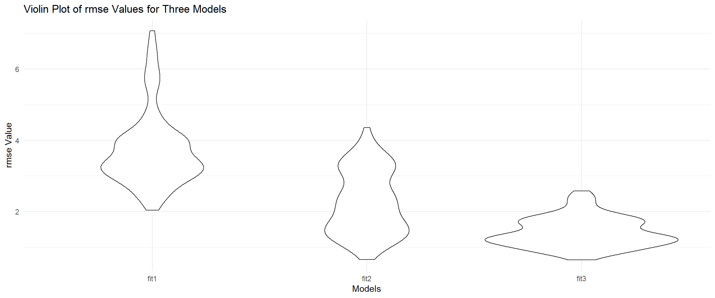
From the violin plot, we can see that model 3 has the lowest rmse, which is the model chosen by forward selection. The first model has only three variables, pld, d, and rank. The second model has four variables, pld, d, rank, and gf. The third model has five variables, pld, d, rank, gf, and ga. After comparing their rmse, we get the final model - w = -1.554369 + 0.661219pld - 0.622216d + 0.015920rank + 0.153794gf -0.225378ga.
Compare the summary of the Models
We use the summary function to compare the R^2 and
p-values of the predictors.
model1=lm(w~pld + d + rank , data = num)
model2=lm(w~pld + d + rank + gf, data = num)
model3=lm(w~pld + d + rank + gf + ga, data = num)
summary(model1)
##
## Call:
## lm(formula = w ~ pld + d + rank, data = num)
##
## Residuals:
## Min 1Q Median 3Q Max
## -9.9168 -1.8090 0.3404 1.8513 10.1195
##
## Coefficients:
## Estimate Std. Error t value Pr(>|t|)
## (Intercept) -6.23478 1.09234 -5.708 0.000000216 ***
## pld 0.80197 0.04533 17.692 < 0.0000000000000002 ***
## d -1.03027 0.20393 -5.052 0.000002986 ***
## rank 0.03749 0.01368 2.740 0.00768 **
## ---
## Signif. codes: 0 '***' 0.001 '**' 0.01 '*' 0.05 '.' 0.1 ' ' 1
##
## Residual standard error: 3.362 on 75 degrees of freedom
## Multiple R-squared: 0.9488, Adjusted R-squared: 0.9468
## F-statistic: 463.6 on 3 and 75 DF, p-value: < 0.00000000000000022summary(model2)##
## Call:
## lm(formula = w ~ pld + d + rank + gf, data = num)
##
## Residuals:
## Min 1Q Median 3Q Max
## -10.0701 -0.3172 0.2980 0.8036 6.7306
##
## Coefficients:
## Estimate Std. Error t value Pr(>|t|)
## (Intercept) -1.687024 0.788267 -2.140 0.0356 *
## pld 0.056613 0.072714 0.779 0.4387
## d -0.065986 0.152813 -0.432 0.6671
## rank 0.007440 0.008861 0.840 0.4038
## gf 0.285927 0.025751 11.103 <0.0000000000000002 ***
## ---
## Signif. codes: 0 '***' 0.001 '**' 0.01 '*' 0.05 '.' 0.1 ' ' 1
##
## Residual standard error: 2.073 on 74 degrees of freedom
## Multiple R-squared: 0.9808, Adjusted R-squared: 0.9798
## F-statistic: 945.5 on 4 and 74 DF, p-value: < 0.00000000000000022summary(model3)##
## Call:
## lm(formula = w ~ pld + d + rank + gf + ga, data = num)
##
## Residuals:
## Min 1Q Median 3Q Max
## -3.8861 -0.5576 0.1279 0.7624 2.3776
##
## Coefficients:
## Estimate Std. Error t value Pr(>|t|)
## (Intercept) -1.560889 0.449031 -3.476 0.00086 ***
## pld 0.660468 0.063756 10.359 0.000000000000000554 ***
## d -0.627753 0.098018 -6.404 0.000000012967977027 ***
## rank 0.015883 0.005092 3.119 0.00259 **
## gf 0.153686 0.018105 8.489 0.000000000001697567 ***
## ga -0.223635 0.017953 -12.456 < 0.0000000000000002 ***
## ---
## Signif. codes: 0 '***' 0.001 '**' 0.01 '*' 0.05 '.' 0.1 ' ' 1
##
## Residual standard error: 1.18 on 73 degrees of freedom
## Multiple R-squared: 0.9939, Adjusted R-squared: 0.9934
## F-statistic: 2363 on 5 and 73 DF, p-value: < 0.00000000000000022By looking at the summary, we can see that model 3 has the highest adj. R^2 of 99.3%, which means our model explain over 99% of the variance in the outcome (wins). This result consists with the result we got from the cross-validation. Therefore, we decide our final model to include 5 variables, pld, d, rank, gf, and ga.
Results/output from regression model
Our final model is w = -1.554369 + 0.661219pld - 0.622216d + 0.015920rank + 0.153794gf -0.225378ga.
After comparing the summary of the three models, we found that the model with variables: pld, d, rank, gf, ga, has the lowest rmse and highest adj.R^2 (about 99%), which means our model explain over 99% of the variance in the outcome (wins). The most significant variable in the model is ga with coefficient of -0.225378. That means if the number of goals scored against a country in the World Cup (since 1990) increases by 1 goal, that would decrease the number of winning by 0.225378, while holding other variables constant.